PyLIMID

Example: promotion and stock decisions

This example models an ice cream shop that chooses whether to run a promotion and how much stock to order. Each kilogram costs $10 and sells for $100, and anything left at closing is thrown away.

The owner has daily sales records and a weather log. From them, the shop estimates a 0.7 probability of a cloudy day and a 0.3 probability of a sunny day, with mean demand of 4 kg on cloudy days and 12 kg on sunny days.

Demand is modeled as a Gamma distribution with concentration 4.0 and rate 4.0 / mean. The concentration gives a coefficient of variation of 0.5. A $60 promotion is expected to raise mean demand by 20%.

The owner announces the promotion the evening before, when tomorrow’s weather is still unknown. In the morning, the owner checks the weather and decides how much to order, remembering whether the promotion is running. The freezer holds up to 40 kg.

The problem can be modeled with the following influence diagram.

The shop is a small example. The same node types and policy families apply to other sequential decisions where the available information and objective can be written down.

Define uncertainty and profit

Demand follows a Gamma distribution whose mean depends on weather and promotion. Profit is revenue from what sells, minus stock and promotion costs.

import jax.numpy as jnp
import numpyro.distributions as dist

from pylimid import (
    ChanceNode,
    DecisionNode,
    DistributionPolicy,
    InfluenceDiagram,
    Interval,
    Linear,
    TabularSoftmax,
    UtilityNode,
    solve,
)

COST = 10.0
PRICE = 100.0
CAPACITY = 40.0
PROMOTION_COST = 60.0
PROMOTION_BOOST = jnp.array([1.0, 1.2])
WEATHER_STATES = ("cloudy", "sunny")
WEATHER_PROBS = jnp.array([0.7, 0.3])
DEMAND_MEANS = jnp.array([4.0, 12.0])

def demand_dist(weather, promotion):
    mean = DEMAND_MEANS[weather] * PROMOTION_BOOST[promotion]
    return dist.Gamma(concentration=4.0, rate=4.0 / mean)


def profit(order, demand, promotion):
    revenue = PRICE * jnp.minimum(order, demand)
    return revenue - COST * order - PROMOTION_COST * promotion

Build the influence diagram

Add the five nodes and connect their dependencies. The promotion chooses between two actions. The order chooses a quantity between 0 and 40 kilograms.

diagram = InfluenceDiagram()
diagram.add_node(
    ChanceNode(
        name="weather",
        states=WEATHER_STATES,
        dist=lambda: dist.Categorical(probs=WEATHER_PROBS),
    )
)
diagram.add_node(
    DecisionNode(
        name="promotion",
        states=("skip", "run"),
        policy_family=TabularSoftmax(),
    )
)
diagram.add_node(
    ChanceNode(name="demand", parents=("weather", "promotion"), dist=demand_dist)
)
diagram.add_node(
    DecisionNode(
        name="order",
        parents=("weather", "promotion"),
        action_space=Interval(0.0, CAPACITY),
        policy_family=DistributionPolicy(
            distribution=dist.TruncatedNormal,
            parameter_model=Linear(outputs=("loc",)),
            fixed_parameters={"low": 0.0, "high": CAPACITY, "scale": 0.25},
        ),
    )
)
diagram.add_node(
    UtilityNode(name="profit", parents=("order", "demand", "promotion"), values=profit)
)

Fit the policies

Fit both policies together, then inspect their estimated expected utility.

solution = solve(diagram, num_steps=2_000)
print(solution.render())

Fitted policies

In this quickstart run, the fitted promotion policy puts more than 99.9% probability on running the promotion. When it runs, mean orders are about 7.2 kg on cloudy days and 21.0 kg on sunny days.

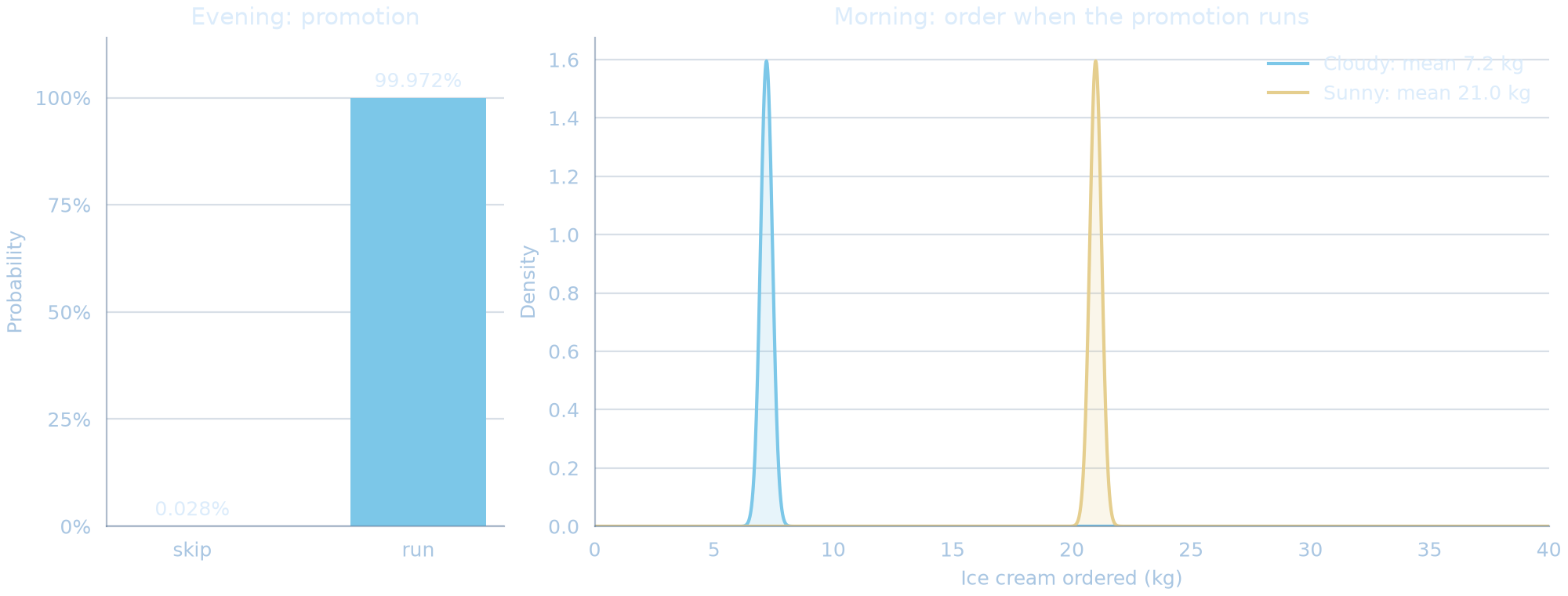
The estimated expected profit is about $542.6 per day. Both fitted policies remain stochastic. Results are approximate, and training does not guarantee the optimal policy.